Kyle's Blog
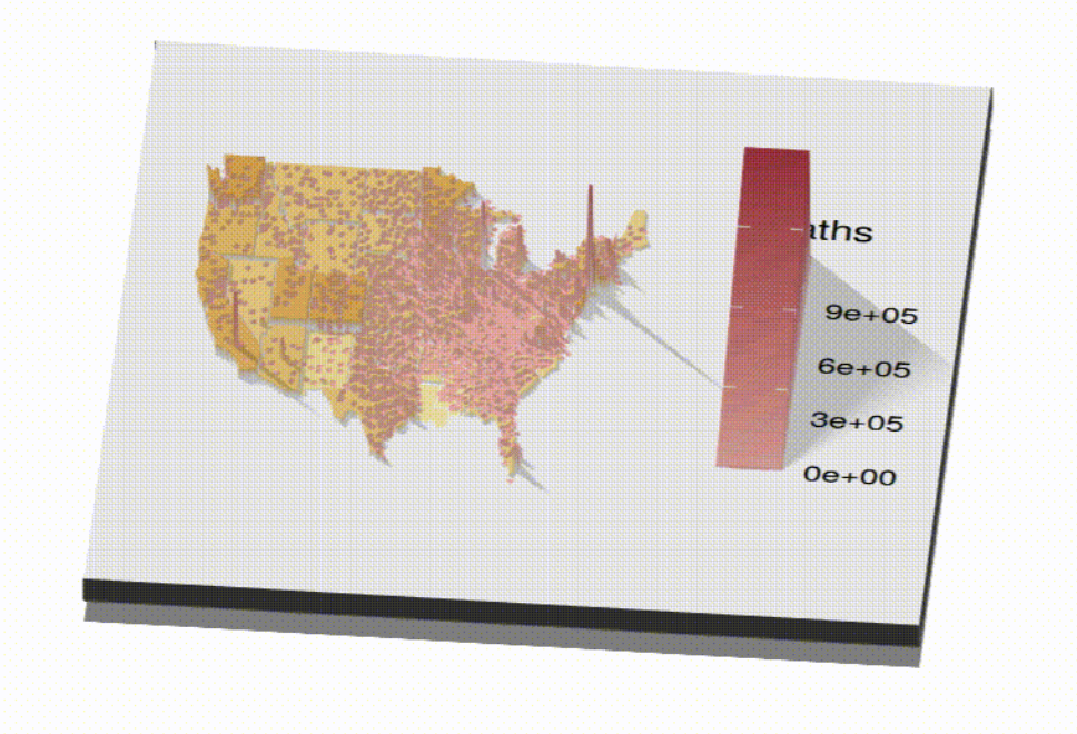
Building a 3D Map in R — Covid Density in the US by Income
Oct, 2020
We are in a golden age of data visualizations AND data!
First, lots of libraries
# Lots of libraries

                    library(sp)

                    library(choroplethrMaps)

                    library(tidyverse)

                    library(tidyverse)

                    library(rgl)

                    library(rayshader)

                    library(png)

                    library(ggplot2)

                    library(grid)

                    library(mapproj)

                    library(av)
Load and preprocess 1st data set
# Preprocess 1st data set

              income = read.csv('income.csv', stringsAsFactors = F)

              income2017 <- income[-c(3:36)]

              income2017$X2017 = as.integer(gsub(',', '', income2017$X2017))

              colNames = c('region', 'value')

              colnames(income2017) <- colNames

              map_outline = data(state.map)

              income2017$region = tolower(income2017$region)

              income2017 <- income2017 %>%  mutate(., region =
              replace(region, region=='d.c.', 'district of columbia') )

              joinedData <- left_join(state.map, income2017, by = 'region')

              keep = c(1,2,3,6,10,13)

              joinedData <- joinedData[, keep]

              map_data = joinedData

              map_data$value = as.numeric(map_data$value)

              map_data <- map_data %>% arrange(., order)

              map_data <- map_data %>% filter(., region != 'alaska')

              map_data <- map_data %>% filter(., region != 'hawaii')
Map
# Map

              map_us = ggplot(map_data, aes(long, lat, group=group, fill =
              value)) +

                geom_polygon() + # Shape

                scale_fill_gradient(limits=range(map_data$value),


              low="#FFF3B0", high="#E09F3E") +

                layer(geom="path", stat="identity", position="identity",

                      mapping=aes(x=long,
              y=lat, group=group,


              color=I('#FFFFFF'))) +

                theme(legend.position = "none",


              axis.line=element_blank(),


              axis.text.x=element_blank(), axis.title.x=element_blank(),


              axis.text.y=element_blank(), axis.title.y=element_blank(),


              axis.ticks=element_blank(),

                      panel.background =
              element_blank()) +

                      coord_map(projection =
              "mercator")

              map_us

              # Save as PNG

              xlim = ggplot_build(map_us)$layout$panel_scales_x[[1]]$range$range

              ylim = ggplot_build(map_us)$layout$panel_scales_y[[1]]$range$range

              ggsave('map_us.png')
Load and map 2nd data set
# Load and map 2nd data set

              covid_df = read.csv('covidbycounty.csv')

              geocode_df = read.csv('geocodedcounties.csv')

              uniqueGeocode <- geocode_df[,-1]

              uniqueCountyGeocode <- unique(uniqueGeocode)

              uniqueCountyGeocode$state_county <-
              paste0(uniqueCountyGeocode$state, uniqueCountyGeocode$county)

              uniqueCountyGeo$county <- paste0(uniqueCountyGeo$county, "
              County")

              uniqueCountyGeo <-
              uniqueCountyGeo[!duplicated(uniqueCountyGeocode$state_county), ]

              covid_df = left_join(covid_df, uniqueCountyGeo[c(2,3,4,5)], by
              =c('county', 'state'))

              covid_df = na.omit(covid_df)

              covid_df <- covid_df %>% filter(., state != 'HI')

              covid_df <- covid_df %>% filter(., state != 'AK')

              map_us_png = readPNG('map_us.png')

              us_covid_deaths = ggplot(covid_df) +

                  annotation_custom(rasterGrob(map_us_png,
              width=unit(1,"npc"), height=unit(1,"npc")),


              -Inf, Inf, -Inf, Inf) + # Background


                 xlim(xlim[1]-2,xlim[2]+1) + # x-axis Mapping

                 ylim(ylim[1]-6,ylim[2]+6.5) + # y-axis Mapping


                geom_point(aes(x=longitude, y=latitude, color=deaths),
              size=0.1) +

                scale_colour_gradient(name = 'deaths',


              limits=range(covid_df$deaths),


              low="#FCB9B2", high="#B23A48") +

                theme(axis.line=element_blank(),


              axis.text.x=element_blank(), axis.title.x=element_blank(),


              axis.text.y=element_blank(), axis.title.y=element_blank(),


              axis.ticks=element_blank(),

                      panel.background =
              element_blank())

              us_covid_deaths

              ggsave('covid_deaths.png')
Make the points 3D and record video
# Make the points 3D and record video

              plot_gg(us_covid_deaths, multicore = TRUE)

              par3d(windowRect = c(0, 0, diff(xlim) * 2500, diff(ylim) * 2500))

              render_camera(fov = 70, zoom = 0.2, theta = 30, phi = 20)

              render_depth(focus = 0.8, focallength = 600)


              phivechalf = 30 + 60 * 1/(1 + exp(seq(-7, 20, length.out =
              180)/2))

              phivecfull = c(phivechalf, rev(phivechalf))

              thetavec = 0 + 45 * sin(seq(0,359,length.out = 360) * pi/180)

              zoomvec = 0.45 + 0.2 * 1/(1 + exp(seq(-5, 20, length.out = 180)))

              zoomvecfull = c(zoomvec, rev(zoomvec))

              render_movie(filename = 'output1', type = "custom", frames =
              360,  phi = phivecfull, zoom = zoomvecfull, theta = thetavec)


              transition_values <- function(from, to, steps = 10, one_way =
              FALSE, type = "cos") {

                if (!(type %in% c("cos", "lin"))){stop("type must be one
              of: 'cos', 'lin'")}

                range <- c(from, to)

                middle <- mean(range)

                half_width <- diff(range)/2

                if (type == "cos") {scaling <- cos(seq(0, 2*pi /
              ifelse(one_way, 2, 1), length.out = steps))}

                else if (type == "lin"){

                  if (one_way) {xout <- seq(1, -1, length.out
              = steps)}

                  else {xout <- c(seq(1, -1, length.out =
              floor(steps/2)), seq(-1, 1, length.out = ceiling(steps/2)))}

                  scaling <- approx(x = c(-1, 1), y = c(-1,
              1), xout = xout)$y }

                middle - half_width * scaling

              }

              theta <- transition_values(from = 0, to = 360, steps = 360,
              one_way = TRUE, type = "lin")

              phi <- transition_values(from = 10, to = 70, steps = 360,
              one_way = FALSE, type = "cos")

              zoom <- transition_values(from = 0.4, to = 0.8, steps = 360,
              one_way = FALSE, type = "cos")

              render_movie(filename = 'output2', type = "custom", frames =
              360,  phi = phi, zoom = zoom, theta = theta)


              rgl.close()