%matplotlib inline
import warnings
import numpy as np
import pandas as pd
import seaborn as sea
import matplotlib.pyplot as plt
from sklearn.impute import SimpleImputer
from sklearn import datasets, linear_model
from sklearn.linear_model import LogisticRegression
from sklearn.model_selection import train_test_split, GridSearchCV
from sklearn.linear_model import LinearRegression, Ridge, Lasso, ElasticNet
from sklearn.ensemble import RandomForestRegressor, GradientBoostingRegressor
from sklearn.neighbors import KNeighborsRegressor
# Ignore the warnings
warnings.filterwarnings('ignore')
# Load the data
train = pd.read_csv('train.csv')
Check For Missing Data
# Check missingness:
missingData = train.isnull().mean(axis=0)
# remove is greater than 30%
# index and gives the column names
missingIndex = missingData[missingData>0.3].index
missingIndex
# Make a working copy of the data
workingDf = train.copy()
workingDf.isna().sum().loc[workingDf.isna().sum()>0].sort_values()
Will output any features with missing data.

Index(['Alley', 'FireplaceQu', 'PoolQC', 'Fence', 'MiscFeature'], dtype='object')
Electrical         1
MasVnrType         8
MasVnrArea         8
BsmtQual          37
BsmtCond          37
BsmtFinType1      37
BsmtExposure      38
BsmtFinType2      38
GarageCond        81
GarageQual        81
GarageFinish      81
GarageType        81
GarageYrBlt       81
LotFrontage      259
FireplaceQu      690
Fence           1179
Alley           1369
MiscFeature     1406
PoolQC          1453
dtype: int64
Much of the missing data is often just because there is no pool or fireplace or whatever, so we can replace NULL’s with 0 or “No Pool”, or whatever the feature. Do this for each feature with something like this:

#Remove NA from PoolQC
workingDf.loc[pd.Series(workingDf.PoolQC.isna()), 'PoolQC'] = 'NoPool'
Some features may be highly correlated AND have missing values. Check correlation with feature you might suspect with something like a scatter plot. For example, LotFrontage is missing a lot of data but my guess is it is correlated to total LotArea.

# Compare frontage to lot area!
lotFrontageByArea = workingDf[['LotFrontage', 'LotArea']]
plt.scatter(np.log(workingDf['LotArea']), np.log(workingDf['LotFrontage']))

Appears Highly Correlated
Now, to fill in missing data from a correlated feature we can make a model of the two, split them into missing and non-missing, then predict the missing values and recombine!

from sklearn.impute import SimpleImputer
from sklearn.linear_model import LinearRegression, Ridge, Lasso, ElasticNet
lotByAreaModel = linear_model.LinearRegression()
lotByAreaModel.fit(lotFrontageNoNa[['LotArea']], lotFrontageNoNa.LotFrontage)
#Spint into missing and not missing
workingDfFrontageNas = workingDf[workingDf.LotFrontage.isna()]
workingDfFrontageNoNas = workingDf[~workingDf.LotFrontage.isna()]
# Must use Data frame
workingDfFrontageNas.LotFrontage = lotByAreaModel.predict(workingDfFrontageNas[['LotArea']])
# Must concat a list!!!
workingDfImputedFrontage = pd.concat([workingDfFrontageNas, workingDfFrontageNoNas], axis = 0)
Next, you will need to dummify the the categorical features. In some cases this can make our data set extremely “wide” but that is ok for most of the regression we will be using.

# Now Dummify to, workingDummies
workingDummies = workingClean.copy()
workingDummies = pd.get_dummies(workingDummies)
print(workingDummies.shape)
workingDummies.head()
print(workingDummies.isna().sum().loc[workingDummies.isna().sum()>0].sort_values(ascending=False))
Make sure you have no NA values.

# Replace NAs in Dummies Set with 0
print(workingDummies.isna().sum().loc[workingDummies.isna().sum()>0].sort_values(ascending=False))
Split your data into training and testing sets:

#split feature and salePrice
salePriceClean = workingClean.SalePrice
homeFeaturesClean = workingClean.copy().drop("SalePrice",axis=1)
salePriceDummies = workingDummies.SalePrice
homeFeaturesDummies=workingDummies.copy().drop("SalePrice",axis=1)
Now, for EDA we will visualize the continuous and categorical features separately. First, here is how to make a grid of histograms for all numeric values.

# Split into contious and Categorical
workingNumeric = workingClean[['GarageYrBlt', 'LotFrontage', 'LotArea', 'OverallCond', 'YearBuilt', 'YearRemodAdd',  'MoSold', 'GarageArea', 'TotRmsAbvGrd', 'GrLivArea', 'BsmtUnfSF', 'MSSubClass', 'YrSold', 'MiscVal', 'BsmtFinSF1', 'BsmtFinSF2', 'TotalBsmtSF', '1stFlrSF', '2ndFlrSF', 'LowQualFinSF', 'BsmtFullBath','BsmtHalfBath', 'FullBath', 'HalfBath', 'BedroomAbvGr', 'KitchenAbvGr', 'Fireplaces', 'GarageCars', 'WoodDeckSF', 'OpenPorchSF','EnclosedPorch', '3SsnPorch', 'ScreenPorch', 'PoolArea', 'OverallQual', 'MasVnrArea']]
workingNumeric['SalePrice'] = salePriceClean
Now, plot with plt.

​fig = plt.figure(figsize=[20,10])
# get current axis = gca
ax = fig.gca()
# We here will apply to the last one described...
workingNumeric.hist(ax = ax)
plt.subplots_adjust(hspace=0.5)

Then we can look at a correlation heat map for these same features:

rs = workingNumeric
d = pd.DataFrame(data=workingNumeric, columns=list(workingNumeric.columns))
# Compute the correlation matrix
corr = d.corr()
# Generate a mask for the upper triangle
mask = np.triu(np.ones_like(corr, dtype=bool))
# Set up the matplotlib figure
f, ax = plt.subplots(figsize=(11, 9))
# Generate a custom diverging colormap
cmap = sea.diverging_palette(230, 20, as_cmap=True)
# Draw the heatmap with the mask and correct aspect ratio
sea.heatmap(corr, mask=mask, cmap=cmap, vmax=.3, center=0,
square=True, linewidths=.5, cbar_kws={"shrink": .5})

Next, this is how we generate a grid of bar charts in Python for all the categorical features. Unfortunately we unlike the boxplot code we need to generate each plot separately and put them in the plot, I will just show code for the first few here.

fig, axes = plt.subplots(13, 3, figsize=(18, 55))
sea.boxplot(ax=axes[0, 0], data=workingCategorical, x='MSZoning', y='SalePrice')
sea.boxplot(ax=axes[0, 1], data=workingCategorical, x='SaleType', y='SalePrice')
sea.boxplot(ax=axes[0, 2], data=workingCategorical, x='GarageType', y='SalePrice')

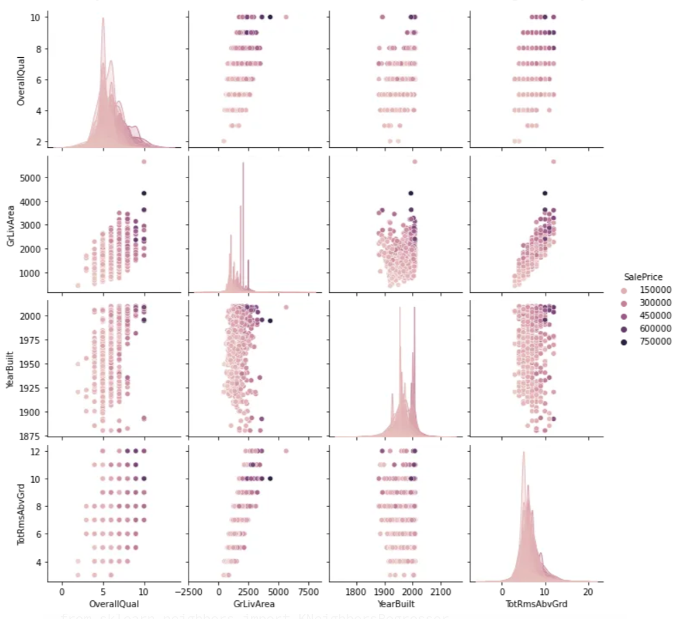
Finally, onto our model building. Here I will show how to do a few regression models with the dummified data set and the results for which was best and how we use that information.

First, the KNN model using grid search to find the best parameters (alpha):

1

#KNN
knn_model = KNeighborsRegressor()
param_grid = {'n_neighbors':np.arange(5, 200, 5)}
gsModelTrain = GridSearchCV(estimator = knn_model, param_grid = param_grid, cv=2)
gsModelTrain.fit(featuresDummiesTrain, priceDummiesTrain)
knn_model.set_params(**gsModelTrain.best_params_)
#fit to train data
knn_model.fit(featuresDummiesTrain, priceDummiesTrain)
#Get scores comparing real house prices and predicted house prices from the test dataset.
print("r2 Test score:", r2_score(priceDummiesTest, knn_model.predict(featuresDummiesTest)))
print("r2 Train score:", r2_score(priceDummiesTrain, knn_model.predict(featuresDummiesTrain)))
trainRMSE = np.sqrt(mean_squared_error(y_true=priceDummiesTrain, y_pred=knn_model.predict(featuresDummiesTrain)))
testRMSE = np.sqrt(mean_squared_error(y_true=priceDummiesTest, y_pred=knn_model.predict(featuresDummiesTest)))
print("Train RMSE:", trainRMSE)
print("Test RMSE:", testRMSE)
The Results!

​r2 Test score: 0.6307760069201898
r2 Train score: 0.7662448448900541
Train RMSE: 37918.53459536937
Test RMSE: 48967.481488778656
Now, do this same exact thing for Ridge(), Lasso, RandomForrest but alter the parameters being optimized for. Here are my final results:


We see the random forest or boosting model was best, so next we grab the most important features from that model, like this:

rfModel.feature_importances_
feature_importances = pd.DataFrame(rfModel.feature_importances_,
index = featuresDummiesTrain.columns,
columns=['importance']).sort_values('importance',ascending=False)
pd.set_option("display.max_rows",None,"display.max_columns",None)
print(feature_importances)
feature_importances.index[:10]
And this is how we get a list of the most important features in this model using Python!

​importance
OverallQual              5.559609e-01
GrLivArea                9.929112e-02
TotalBsmtSF              4.050054e-02
1stFlrSF                 3.604577e-02
TotRmsAbvGrd             2.772576e-02
FullBath                 2.693519e-02
BsmtFinSF1               2.064975e-02
GarageCars               1.915783e-02
2ndFlrSF                 1.753713e-02
GarageArea               1.748563e-02
LotArea                  1.219073e-02
YearBuilt                1.075511e-02
LotFrontage              7.270100e-03
YearRemodAdd             7.038709e-03
BsmtQual_Ex              5.726935e-03
OpenPorchSF              4.677578e-03
BsmtUnfSF                4.245650e-03
MoSold                   3.397142e-03
OverallCond              3.180477e-03
WoodDeckSF               2.865491e-03
KitchenQual_Gd           2.692117e-03
ExterQual_Ex             2.253200e-03
GarageType_Detchd        1.832978e-03
MSSubClass               1.808349e-03
BsmtFullBath             1.791505e-03
MSZoning_RM              1.781576e-03
ScreenPorch              1.679301e-03
YrSold                   1.664580e-03
BsmtExposure_No          1.533721e-03
GarageFinish_Unf         1.514469e-03
MasVnrArea_1170.0        1.431316e-03
So now we know that the overall quality of a home along with its size is very important but we can basically ignore things like a finished garage or if it has a screened in porch or not!

You can use this same system to evaluate any home data with any number of features. Our big take away here is that all the features on the bottom of this list can be safely ignored so if you are selling or pricing a home there is no reason to even take them into account most of the time.

Happy house hunting and thank you!